1: Random Forests - Intermediate Data Programming

What is XGBoost?¶

For this series of lessons we will be learning about XGBoost. First lets take a look at where we are headed and the features of XGBoost.

Random Forests¶

In this lesson, we’ll discover why a single decision tree can be unreliable and how random forests fix this by combining many trees together. We’ll use California housing price data to observe the problem firsthand, build intuition for the solution, and then apply sklearn’s RandomForestRegressor.

Learning Objectives¶

By the end of this lesson, students will be able to:

Explain why a single decision tree suffers from high variance and overfitting
Describe how bootstrap sampling and bagging reduce variance through averaging
Apply RandomForestRegressor and RandomForestClassifier from sklearn
Interpret feature importance scores to identify which variables most drive predictions

Introduction: The California Housing Problem¶

In our machine learning lesson, we saw how decision trees learn a nested if-then-else hierarchy to make predictions — we used them to classify houses as NY or SF and to calibrate air quality sensor data.

But in data science, knowing a model’s weaknesses is just as important as knowing its strengths.

In this lesson, we’ll work with a dataset from the 1990 U.S. Census that contains information about 20,640 housing districts (census block groups) across California. Our goal is to predict the median house value for each district from features like income, house age, and location.

This kind of prediction has real-world value: real estate analysts use it to find undervalued properties, city planners use it to study housing affordability, and researchers use it to track economic inequality.

What a Decision Tree Looks Like¶

A decision tree makes predictions with a sequence of yes/no questions, assigning a score at each leaf. The diagram below — a Classification and Regression Tree (CART) — predicts how much a person would enjoy a hypothetical computer game from features like age and gender. Each leaf holds a real-valued score, not just a class label, which is what lets us add trees together later.

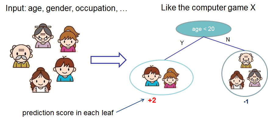
Image: XGBoost documentation — Introduction to Boosted Trees. This is exactly the kind of tree DecisionTreeRegressor builds for our housing data — just with many more splits.

import pandas as pd
import numpy as np
import seaborn as sns
import matplotlib.pyplot as plt
from sklearn.datasets import fetch_california_housing
sns.set_theme()

housing = fetch_california_housing(as_frame=True)
df = housing.frame
df.head()

The dataset contains 8 features and one target variable:

Feature	Description
`MedInc`	Median income in block group (in $10,000s)
`HouseAge`	Median house age in block group (years)
`AveRooms`	Average number of rooms per household
`AveBedrms`	Average number of bedrooms per household
`Population`	Block group population
`AveOccup`	Average number of household members
`Latitude`	Block group latitude
`Longitude`	Block group longitude
`MedHouseVal`	Target: Median house value in $100,000s

Before building a model, which feature do you think will be the strongest predictor of house value? What’s your intuition?

# Visualize the relationship between income and house value
sns.relplot(df, x="MedInc", y="MedHouseVal", alpha=0.15)

The scatter plot confirms a positive relationship: wealthier districts have more expensive homes. Notice the hard ceiling at 5.0 ($500,000) — values above this were clipped in the original data, which will affect model predictions at the high end.

The Variance Problem¶

Let’s train a decision tree, split the data 80/20 into training and testing sets, and measure the root mean squared error (RMSE) — lower is better. (It’s actually the “Quadratic Mean Error” or “Root-Mean-Square Deviation” but we simplify with average prediction error here)

from sklearn.model_selection import train_test_split
from sklearn.tree import DecisionTreeRegressor
from sklearn.metrics import root_mean_squared_error

X = df.drop("MedHouseVal", axis=1)
y = df["MedHouseVal"]

X_train, X_test, y_train, y_test = train_test_split(X, y, test_size=0.2, random_state=42)

tree = DecisionTreeRegressor(max_depth=5, random_state=42)
tree.fit(X_train, y_train)
rmse = root_mean_squared_error(y_test, tree.predict(X_test))
print(f"Test RMSE: {rmse:.4f}  (≈ ${rmse * 100_000:,.0f} average prediction error)")

Now here’s a critical question: what happens if we train the exact same model with the exact same hyperparameters, but on a slightly different split of the data?

# Train the same tree on 6 different random splits
print("Testing variance across different data splits:\n")
rmses = []
for seed in range(6):
    X_tr, X_te, y_tr, y_te = train_test_split(X, y, test_size=0.2, random_state=seed)
    t = DecisionTreeRegressor(max_depth=5, random_state=0).fit(X_tr, y_tr)
    rmse = root_mean_squared_error(y_te, t.predict(X_te))
    rmses.append(rmse)
    print(f"  Split {seed}: RMSE = {rmse:.4f}")

print(f"\nRange across splits: {max(rmses) - min(rmses):.4f}")

The RMSE shifts noticeably depending on which data ends up in the training set. This is called high variance: the model’s performance swings significantly based on the particular training sample it received.

An even more telling sign of high variance is looking at what happens when a model overfits. We can see this clearly by comparing training error vs. testing error with an unlimited-depth tree:

# An unrestricted tree can memorize the training data perfectly
big_tree = DecisionTreeRegressor(random_state=42)
big_tree.fit(X_train, y_train)

print("Train RMSE:", root_mean_squared_error(y_train, big_tree.predict(X_train)))
print("Test  RMSE:", root_mean_squared_error(y_test,  big_tree.predict(X_test)))

Near-zero training error with much higher test error is the hallmark of overfitting: the tree has memorized noise in the training data rather than learning generalizable rules.

Note: The gap between train error and test error is just as important as the absolute values. A model with 0.0 train RMSE and ~0.7 test RMSE is overfit — it performs perfectly on data it has seen but poorly on new data.

Bagging: The Wisdom of Crowds¶

The fix for high variance comes from a simple insight: average many noisy estimates to get one stable estimate.

Imagine asking 500 people to independently guess the weight of a jar of coins. Each person’s guess is imprecise (high variance), but the average of all 500 guesses is remarkably close to the true weight. This “wisdom of crowds” effect is the foundation of bagging (Bootstrap Aggregating).

How bagging works:

Create n different training sets by sampling with replacement from the original data (each such sample is called a bootstrap sample)
Train a separate decision tree on each bootstrap sample
To make a prediction, run all n trees and average their predictions (for regression) or take a majority vote (for classification)

Each tree makes different mistakes because it saw different training data. Those individual errors tend to cancel out when averaged together.

from sklearn.utils import resample

n_trees = 50
all_predictions = []

for i in range(n_trees):
    # Bootstrap: sample with replacement (same size as training set)
    X_boot, y_boot = resample(X_train, y_train, random_state=i)
    t = DecisionTreeRegressor(random_state=i)
    t.fit(X_boot, y_boot)
    all_predictions.append(t.predict(X_test))

# Average predictions across all 50 trees
bagged_pred = np.mean(all_predictions, axis=0)
print(f"Single tree RMSE:  {root_mean_squared_error(y_test, big_tree.predict(X_test)):.4f}")
print(f"Bagged trees RMSE: {root_mean_squared_error(y_test, bagged_pred):.4f}")

A large improvement! By averaging 50 trees, the individual errors cancel out and we get a much more accurate and stable model.

Random Forests¶

Random forests add one more powerful twist to bagging: at each split in each tree, instead of considering all features, we only look at a random subset of features.

Without this restriction, all trees tend to make the same early splits (e.g., always split on MedInc first since it’s the most predictive). This creates correlated trees, and averaging correlated predictions doesn’t reduce variance much. By forcing trees to choose from a random subset of features, the trees become more diverse and decorrelated — their average is far more reliable.

sklearn’s RandomForestRegressor implements this efficiently:

Visualizing an ensemble. Instead of trusting one tree, an ensemble combines many. The diagram below shows two trees whose leaf scores are added together to form the final prediction — each tree captures part of the signal that the other misses:

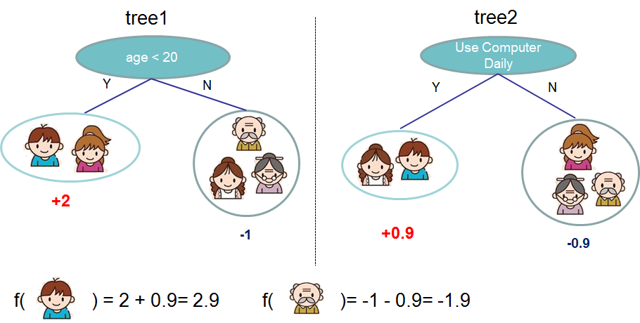
Image: XGBoost documentation — Introduction to Boosted Trees. A random forest combines trees by averaging (rather than summing) their predictions, but the idea is the same: many trees beat one.

from sklearn.ensemble import RandomForestRegressor

rf = RandomForestRegressor(n_estimators=100, random_state=42, n_jobs=-1)
rf.fit(X_train, y_train)
print(f"Random Forest RMSE: {root_mean_squared_error(y_test, rf.predict(X_test)):.4f}")

Key hyperparameters for random forests:

Hyperparameter	What it controls	Default
`n_estimators`	Number of trees in the forest	`100`
`max_depth`	Maximum depth of each tree	`None` (fully grown)
`max_features`	Features to consider at each split	`"sqrt"`
`min_samples_leaf`	Minimum samples required at each leaf	`1`
`n_jobs`	CPU cores to use (`-1` = all)	`1`

Does adding more trees always help? Is there a point of diminishing returns?

# Note - this will take a few minutes to run with 300 trees
n_values = [1, 5, 10, 25, 50, 100, 200, 300]
rmse_by_n = []

for n in n_values:
    rf_n = RandomForestRegressor(n_estimators=n, random_state=42, n_jobs=-1)
    rf_n.fit(X_train, y_train)
    rmse_by_n.append(root_mean_squared_error(y_test, rf_n.predict(X_test)))

sns.lineplot(x=n_values, y=rmse_by_n, marker="o")
plt.xlabel("Number of Trees (n_estimators)")
plt.ylabel("Test RMSE")
plt.title("Effect of Forest Size on Prediction Error");

Feature Importance¶

One of the most valuable properties of random forests is feature importance: a measure of how much each variable contributed to reducing prediction error across all splits in all trees. A higher importance score means the model relies more heavily on that feature.

importance_df = pd.DataFrame({
    "Feature": X.columns,
    "Importance": rf.feature_importances_
}).sort_values("Importance", ascending=True)

sns.barplot(importance_df, x="Importance", y="Feature", orient="h")
plt.title("Random Forest Feature Importances")
plt.xlabel("Mean Decrease in Impurity")
plt.tight_layout();

Were your earlier predictions about feature importance correct? What might explain why MedInc and location features (Latitude, Longitude) dominate?

Summary¶

Model	Strategy	Approx. Test RMSE
Decision Tree (max_depth=5)	Single tree	~0.73
Decision Tree (no limit)	Overfit single tree	~0.73
Bagged Trees (50 trees)	Average bootstrap-trained trees	~0.52
Random Forest (100 trees)	Bagging + feature randomness	~0.50

Key takeaways:

Single decision trees have high variance — they overfit and change with different training data
Bagging reduces variance by training many trees on bootstrap samples and averaging
Random forests further reduce variance by randomizing which features each tree considers at each split, creating diverse, decorrelated trees
Feature importances reveal which variables drive predictions

In the next lesson, we’ll learn about a fundamentally different strategy for combining trees — one that produces even better predictions by learning from mistakes.

Practice Problems¶

Problem 1¶

The California housing dataset is a regression problem. Apply what you’ve learned to a classification task: predicting whether a tumor is malignant (0) or benign (1) from clinical measurements.

Load load_breast_cancer, train a RandomForestClassifier, and compare its accuracy to a single DecisionTreeClassifier.

from sklearn.datasets import load_breast_cancer
from sklearn.ensemble import RandomForestClassifier
from sklearn.tree import DecisionTreeClassifier
from sklearn.metrics import accuracy_score

cancer = load_breast_cancer(as_frame=True)
df_cancer = cancer.frame
X_c = df_cancer.drop("target", axis=1)
y_c = df_cancer["target"]

X_c_train, X_c_test, y_c_train, y_c_test = train_test_split(
    X_c, y_c, test_size=0.2, random_state=42
)

# TODO: Train a RandomForestClassifier with 100 trees
clf_rf = ...
clf_rf.fit(...)

# TODO: Train a single DecisionTreeClassifier for comparison
clf_dt = ...
clf_dt.fit(...)

print("Random Forest Accuracy:", accuracy_score(y_c_test, clf_rf.predict(X_c_test)))
print("Decision Tree Accuracy:", accuracy_score(y_c_test, clf_dt.predict(X_c_test)))

Problem 2¶

Fill in the code below to investigate how max_depth affects both training and test RMSE for a random forest on the California housing data. Use depths from 2 to 15.

At what depth does overfitting begin? How does the “safe” depth for a random forest compare to a single decision tree? Why might they differ?

depths = list(range(2, 16))
train_rmses = []
test_rmses  = []

for depth in depths:
    # TODO: Create a RandomForestRegressor with n_estimators=50 and max_depth=depth
    rf_d = ...
    rf_d.fit(X_train, y_train)
    train_rmses.append(root_mean_squared_error(y_train, rf_d.predict(X_train)))
    test_rmses.append( root_mean_squared_error(y_test,  rf_d.predict(X_test)))

results = pd.DataFrame({
    "max_depth": depths * 2,
    "RMSE": train_rmses + test_rmses,
    "Split": ["Train"] * len(depths) + ["Test"] * len(depths)
})
sns.lineplot(results, x="max_depth", y="RMSE", hue="Split")
plt.title("Train vs. Test RMSE by max_depth")
plt.xlabel("max_depth");

Key Takeaway Random Forest Depth & Overfitting

While a single decision tree overfits catastrophically (causing test error to actively shoot back up), a Random Forest’s test error plateaus instead.

Where it begins: Overfitting starts when you see the train / test errors diverge. Beyond this point, the training error continues to plummet while the test error completely flattens out.

Why it’s “safe”: Because Random Forests average many independent, randomized trees, the individual overfitting errors cancel out. This means you don’t aggressively penalize test accuracy by setting the depth too high, though it will cost you extra memory and compute time!

Problem 3¶

Feature importance showed that AveOccup, Population, and AveBedrms contribute very little. Train a random forest using only the 4 most important features. How much does restricting features hurt performance?

Using fewer features is called feature selection — a simpler model that performs comparably is often preferred because it’s faster, cheaper to collect data for, and easier to explain.

# Retrieve top-4 features from the importance DataFrame above
top_4 = importance_df.sort_values("Importance", ascending=False)["Feature"].head(4).tolist()
print("Top 4 features:", top_4)

# TODO: Train a RandomForestRegressor on only these 4 features
rf_small = ...
rf_small.fit(...)

print(f"Full model RMSE    (8 features): "
      f"{root_mean_squared_error(y_test, rf.predict(X_test)):.4f}")
print(f"Reduced model RMSE (4 features): "
      f"{root_mean_squared_error(y_test, rf_small.predict(X_test[top_4])):.4f}")