3: Hyperparameter Tuning - Intermediate Data Programming

In the last two lessons, we’ve been using XGBoost with mostly default parameters or hand- picked values. In this lesson, we’ll learn what XGBoost’s key parameters actually control and how to find the best combination systematically using cross-validation and grid search.

Learning Objectives¶

By the end of this lesson, students will be able to:

Identify the key XGBoost hyperparameters and explain their effect on model behavior
Apply cross_val_score to evaluate models without using the test set
Use GridSearchCV to automatically find the best hyperparameter combination
Compare XGBoost’s three built-in feature importance methods

try:
    import xgboost
except ImportError:
    %pip install xgboost
import pandas as pd
import numpy as np
import seaborn as sns
import matplotlib.pyplot as plt
from sklearn.datasets import fetch_california_housing, load_breast_cancer
from sklearn.model_selection import train_test_split, cross_val_score, GridSearchCV
from sklearn.metrics import root_mean_squared_error, accuracy_score
from xgboost import XGBRegressor, XGBClassifier
sns.set_theme()

# Regression dataset (California housing)
housing = fetch_california_housing(as_frame=True)
df = housing.frame
X_reg = df.drop("MedHouseVal", axis=1)
y_reg = df["MedHouseVal"]
X_r_tr, X_r_te, y_r_tr, y_r_te = train_test_split(
    X_reg, y_reg, test_size=0.2, random_state=42)

# Classification dataset (Breast cancer)
cancer = load_breast_cancer(as_frame=True)
df_c = cancer.frame
X_clf = df_c.drop("target", axis=1)
y_clf = df_c["target"]
X_c_tr, X_c_te, y_c_tr, y_c_te = train_test_split(
    X_clf, y_clf, test_size=0.2, random_state=42)

print("Regression dataset:", X_reg.shape)
print("Classification dataset:", X_clf.shape)

XGBoost Hyperparameter Overview¶

XGBoost has many parameters. We’ll focus on the ones that matter most in practice:

Parameter	Category	Default	Effect
`n_estimators`	Boosting	`100`	Number of trees; more = slower but potentially better
`learning_rate`	Boosting	`0.3`	Shrinkage per tree; lower = more stable
`max_depth`	Tree	`6`	Max tree depth; deeper = more complex, more prone to overfit
`min_child_weight`	Tree	`1`	Minimum sum of weights in a leaf; higher = more conservative
`subsample`	Sampling	`1.0`	Fraction of rows sampled per tree
`colsample_bytree`	Sampling	`1.0`	Fraction of columns sampled per tree
`reg_alpha`	Regularization	`0`	L1 penalty on weights; sparse solutions
`reg_lambda`	Regularization	`1`	L2 penalty on weights; shrinks weights toward zero

These parameters can be grouped into three categories:

Boosting parameters — control the learning process
Tree parameters — control individual tree complexity
Regularization parameters — prevent overfitting

Let’s explore each group.

Boosting Parameters: Learning Rate and n_estimators¶

learning_rate and n_estimators always work together. A smaller learning rate means each tree makes a tinier correction, so you need more trees to reach the same total correction. The relationship is roughly:

Total effect ≈ learning_rate × n_estimators

A common strategy is to set a small learning_rate (e.g., 0.05 or 0.01) and let n_estimators be tuned — you’ll usually get a better model than with a high learning rate.

The chart below illustrates this trade-off:

configs = [
    (0.30,  50), (0.30, 100), (0.30, 200),
    (0.10,  50), (0.10, 100), (0.10, 200),
    (0.05,  50), (0.05, 100), (0.05, 200),
    (0.01,  50), (0.01, 100), (0.01, 200),
]
# Uncomment the follwoing to run with more configurations (takes longer to run)
# This will show you how the learning rate at 001 can outperform when we have even more trees
# configs = [
#     (0.30,  50), (0.30, 100), (0.30, 200), (0.3, 3000),
#     (0.10,  50), (0.10, 100), (0.10, 200), (0.1, 3000),
#     (0.05,  50), (0.05, 100), (0.05, 200), (0.05, 3000),
#     (0.01,  50), (0.01, 100), (0.01, 200), (0.01, 3000),
# ]

rows = []
for lr, n in configs:
    m = XGBRegressor(learning_rate=lr, n_estimators=n, max_depth=6,
                     random_state=42, verbosity=0).fit(X_r_tr, y_r_tr)
    rows.append({
        "learning_rate": str(lr),
        "n_estimators": n,
        "RMSE": root_mean_squared_error(y_r_te, m.predict(X_r_te))
    })

results_lr = pd.DataFrame(rows)
sns.lineplot(results_lr, x="n_estimators", y="RMSE", hue="learning_rate", marker="o")
plt.title("Learning Rate vs. n_estimators Trade-off")
plt.xlabel("n_estimators");

Tree Parameters: Depth and min_child_weight¶

max_depth controls how complex each individual tree is. Shallower trees are less likely to overfit but may underfit; deeper trees capture more signal but can memorize noise.

min_child_weight requires that each leaf node contains at least this much “weight” (the sum of second-order gradient statistics, approximately the number of samples for regression). Higher values create more conservative trees with fewer splits.

How a tree decides where to split. To grow a tree, XGBoost sorts the data on each feature and scans left-to-right, scoring every possible split point and keeping the best one. max_depth caps how many times this can happen down a branch, and min_child_weight blocks splits that would leave too little data in a leaf:

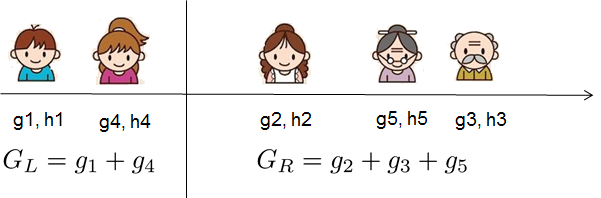
Image: XGBoost documentation — Introduction to Boosted Trees. A single sorted scan evaluates all candidate splits; the tree parameters below constrain which splits are even allowed.

# Heatmap of max_depth vs min_child_weight
depths = [3, 6, 12, 24, 48, 200]
min_cws = [1, 3, 6, 12, 24, 48, 200]

matrix = np.zeros((len(depths), len(min_cws)))
for i, d in enumerate(depths):
    for j, mcw in enumerate(min_cws):
        m = XGBRegressor(max_depth=d, min_child_weight=mcw, n_estimators=100,
                         learning_rate=0.1, random_state=42, verbosity=0)
        m.fit(X_r_tr, y_r_tr)
        matrix[i, j] = root_mean_squared_error(y_r_te, m.predict(X_r_te))

heatmap_df = pd.DataFrame(matrix, index=depths, columns=min_cws)
sns.heatmap(heatmap_df, annot=True, fmt=".3f", cmap="YlOrRd_r",
            xticklabels=min_cws, yticklabels=depths)
plt.xlabel("min_child_weight")
plt.ylabel("max_depth")
plt.title("Test RMSE by max_depth and min_child_weight");

Looking at the heatmap, what combination of max_depth and min_child_weight produces the lowest test RMSE? What does this suggest about the right level of complexity for this dataset?

This combination suggests that the dataset has a high level of underlying complexity, but requires strong regularization to prevent overfitting to noise.

The high max_depth indicates that the model needs the flexibility to build long, multi-step decision paths to capture complex, non-linear relationships in the features. Shallow trees underfit the data.

The high min_child_weight acts as a strict safeguard. It prevents those deep trees from isolating tiny, noisy anomalies. By demanding a high number of samples to justify every split, the model only builds deep branches where there are large, consistent clusters of data to support them. If we don’t increase this sufficiently the tree will start to overfit and increase the RMSE as you can see in the third column where we left this as a lower value.

Regularization: reg_alpha and reg_lambda¶

Regularization adds a penalty to the model for having large weights. It’s a way to discourage complexity and prevent overfitting.

reg_lambda (L2): penalizes large weights — shrinks them toward zero smoothly
reg_alpha (L1): can force weights to exactly zero — useful for feature selection

By default, XGBoost uses L2 regularization (reg_lambda=1). In most cases, you only need to tune these if you’re seeing overfitting that max_depth and min_child_weight don’t fix.

Where regularization enters. XGBoost scores each candidate tree with a structure score that rewards fitting the data but penalizes complexity. The penalty includes reg_lambda (λ, which shrinks leaf scores) and a per-leaf cost. The picture below shows how the gradient statistics at each leaf are combined into that score:

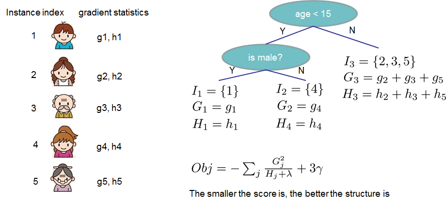
Image: XGBoost documentation — Introduction to Boosted Trees. Larger reg_lambda makes the denominator bigger, pulling every leaf score toward zero — this is the L2 penalty we explore below.

# Effect of reg_lambda on train vs. test error
lambdas = [0, 0.01, 0.1, 1, 5, 10, 50]
train_rmses, test_rmses = [], []

for lam in lambdas:
    m = XGBRegressor(reg_lambda=lam, n_estimators=100, learning_rate=0.1,
                     max_depth=6, random_state=42, verbosity=0)
    m.fit(X_r_tr, y_r_tr)
    train_rmses.append(root_mean_squared_error(y_r_tr, m.predict(X_r_tr)))
    test_rmses.append( root_mean_squared_error(y_r_te, m.predict(X_r_te)))

lam_results = pd.DataFrame({
    "reg_lambda": lambdas * 2,
    "RMSE": train_rmses + test_rmses,
    "Split": ["Train"] * len(lambdas) + ["Test"] * len(lambdas)
})
sns.lineplot(lam_results, x="reg_lambda", y="RMSE", hue="Split", marker="o")
plt.xscale("symlog")
plt.title("Effect of L2 Regularization on Train vs. Test Error")
plt.xlabel("reg_lambda (log scale)");

The Effect of L2 Regularization plot shows that the dataset benefits from smoothing out extreme predictions. It proves that instead of letting individual leaves make huge, confident leaps to fit complex points, the model performs much better on unseen data when each tree is forced to make small, highly conservative, incremental adjustments.

Subsampling Parameters¶

subsample and colsample_bytree introduce randomness similar to random forests:

subsample: each tree only sees a random fraction of the training rows
colsample_bytree: each tree only uses a random fraction of the features

These help prevent overfitting by adding noise that keeps the model from memorizing specific data points, and they also make training faster.

# Effect of subsample on performance
samples = [0.5, 0.6, 0.7, 0.8, 0.9, 1.0]
train_rmses, test_rmses = [], []

for s in samples:
    m = XGBRegressor(subsample=s, colsample_bytree=0.8, n_estimators=100,
                     learning_rate=0.1, max_depth=6, random_state=42, verbosity=0)
    m.fit(X_r_tr, y_r_tr)
    train_rmses.append(root_mean_squared_error(y_r_tr, m.predict(X_r_tr)))
    test_rmses.append( root_mean_squared_error(y_r_te, m.predict(X_r_te)))

sub_results = pd.DataFrame({
    "subsample": samples * 2,
    "RMSE": train_rmses + test_rmses,
    "Split": ["Train"] * len(samples) + ["Test"] * len(samples)
})
sns.lineplot(sub_results, x="subsample", y="RMSE", hue="Split", marker="o")
plt.title("Effect of subsample on Train vs. Test Error")
plt.xlabel("subsample fraction");

The plot shows that a subsample rate of 1.0 yields the lowest Test RMSE, indicating that the model performs best when trained on the full dataset rather than a random subset. The jagged fluctuations at lower subsample values reflect the random variance introduced by stochastic sampling. Because the model is already heavily regularized by parameters like min_child_weight, dropping the subsample rate below 1.0 merely deprives the model of valuable data points without providing any additional defensive benefit.

Cross-Validation: Using the Training Set Wisely¶

In Model Evaluation, we learned that the test set must only be used once — at the very end, to report the final model’s performance. If we keep testing different hyperparameters against the test set, we’re essentially training on the test set.

Cross-validation is the solution: split the training set into k folds. For each fold, train on the other k-1 folds and evaluate on the held-out fold. Average the k scores to estimate true performance.

To understand cross-validation, it helps to first look at the flaw of the standard approach you often see in machine learning: the simple Train/Test split.

When you split your data just once (say, 80% training and 20% testing), you run into a major gamble: What if your 20% test set happens to contain mostly easy-to-predict data points? Or mostly weird outliers? Your test score will fluctuate wildly depending on how the random number generator sliced the data that morning.

Cross-validation is the industry-standard fix for this. It is a systematic way to ensure every single data point gets a turn to be part of the test set.

cross_val_score automates this:

from sklearn.model_selection import cross_val_score

# Use cross-validation (5 folds) to estimate test performance WITHOUT touching X_r_te
xgb_cv = XGBRegressor(n_estimators=100, learning_rate=0.1, max_depth=6,
                      random_state=42, verbosity=0)

cv_scores = cross_val_score(
    estimator=xgb_cv,
    X=X_r_tr,
    y=y_r_tr,
    scoring="neg_root_mean_squared_error",
    cv=5,
    verbose=1
)

print("CV scores (neg RMSE):", cv_scores)
print(f"Mean CV RMSE: {-cv_scores.mean():.4f} ± {cv_scores.std():.4f}")

GridSearchCV: Automating Hyperparameter Search¶

Rather than manually testing every combination of parameters, GridSearchCV does it automatically using cross-validation. It exhaustively tries every combination in the parameter grid and returns the best one.

Note: The test set X_r_te / y_r_te is never touched during GridSearchCV. We only use the training data here. The test set is reserved for our final evaluation.

from sklearn.model_selection import GridSearchCV

param_grid = {
    "max_depth":        [3, 4, 5, 6],
    "learning_rate":    [0.05, 0.10, 0.20],
    "min_child_weight": [1, 3, 5],
}

search = GridSearchCV(
    estimator=XGBRegressor(n_estimators=200, subsample=0.8,
                           colsample_bytree=0.8, random_state=42, verbosity=0),
    param_grid=param_grid,
    scoring="neg_root_mean_squared_error",
    cv=5,
    verbose=2,
    n_jobs=-1
)
search.fit(X_r_tr, y_r_tr)

print("\nBest parameters:", search.best_params_)
print(f"Best CV RMSE:    {-search.best_score_:.4f}")

# Final evaluation: apply the best model to the test set (only once!)
best_model = search.best_estimator_
final_rmse = root_mean_squared_error(y_r_te, best_model.predict(X_r_te))
print(f"Final Test RMSE: {final_rmse:.4f}")

Why might the final test RMSE differ from the best CV RMSE? Is a larger or smaller gap concerning?

When we use Cross-Validation to search a hyperparameter grid, the selection process chooses the specific parameters that performed best on those specific validation folds. Because the model was optimized against the CV folds, the CV score can be slightly overly optimistic. The final test set, however, represents completely unseen, locked-away data that played absolutely no role in choosing the hyperparameters, reflecting a completely unbiased evaluation.

Feature Importance in XGBoost¶

XGBoost provides three different types of feature importance, which can give different rankings:

Type	What it measures
`weight`	Number of times a feature is used in a split
`gain`	Average improvement in loss when a feature is used for a split
`cover`	Average number of samples affected by splits on a feature

gain is generally the most informative because it directly measures how much each feature contributes to reducing the loss.

fig, axes = plt.subplots(1, 3, figsize=(15, 5))
importance_types = ["weight", "gain", "cover"]

for ax, imp_type in zip(axes, importance_types):
    imp = best_model.get_booster().get_score(importance_type=imp_type)
    imp_df = pd.DataFrame(imp.items(), columns=["Feature", "Importance"])
    imp_df = imp_df.sort_values("Importance", ascending=True).tail(8)
    ax.barh(imp_df["Feature"], imp_df["Importance"])
    ax.set_title(f"Importance type: {imp_type}")
    ax.set_xlabel("Score")

plt.suptitle("XGBoost Feature Importance by Type", fontsize=14)
plt.tight_layout();

Do the three importance types agree on which features are most important? What might explain differences between weight and gain?

A feature can have a low weight but high gain if it is used rarely but is incredibly powerful when it is used. Conversely, a feature can have a high weight but low gain if the model uses it constantly for minor, micro-adjustments at the deep, noisy edges of the trees.

Summary¶

Parameter Group	Key Parameters	What to tune
Boosting	`learning_rate`, `n_estimators`	Start with small LR (0.05–0.1), tune n_estimators
Tree structure	`max_depth`, `min_child_weight`	Usually 3–6 depth; higher min_child_weight for noisy data
Regularization	`reg_lambda`, `reg_alpha`	Usually only needed if other methods don’t fix overfit
Subsampling	`subsample`, `colsample_bytree`	Values 0.7–0.9 often help generalization

Workflow for tuning XGBoost:

Fix a small learning_rate (0.05 or 0.1) and a large enough n_estimators
Tune tree structure parameters (max_depth, min_child_weight) via GridSearchCV + CV
Tune subsampling parameters
Optionally tune regularization
Evaluate final model on the test set (once!)

Practice Problems¶

Problem 1¶

Use GridSearchCV on the breast cancer classification dataset to find the best combination of max_depth and learning_rate for an XGBClassifier. Use accuracy as the scoring metric.

from sklearn.model_selection import GridSearchCV

param_grid_c = {
    "max_depth":     [2, 3, 4, 5],
    "learning_rate": [0.05, 0.10, 0.20],
}

search_c = GridSearchCV(
    # TODO: fill in XGBClassifier with appropriate base parameters
    estimator=...,
    param_grid=param_grid_c,
    scoring="accuracy",
    cv=5,
    n_jobs=-1
)
# TODO: fit search_c on X_c_tr, y_c_tr
search_c.fit(...)

print("Best params:", search_c.best_params_)
print(f"Best CV accuracy: {search_c.best_score_:.4f}")
print(f"Final test accuracy: {accuracy_score(y_c_te, search_c.predict(X_c_te)):.4f}")

Problem 2¶

Use cross_val_score to compare three regularization settings on the California housing data: no regularization (reg_lambda=0), default (reg_lambda=1), and strong regularization (reg_lambda=10). Use 5-fold cross-validation with negative RMSE.

Which setting produces the best cross-validated performance? What does this suggest about the role of regularization on this dataset?

reg_lambdas = [0, 1, 10]

for lam in reg_lambdas:
    # TODO: Create XGBRegressor with this reg_lambda and run cross_val_score
    model = ...
    scores = cross_val_score(model, X_r_tr, y_r_tr,
                             scoring="neg_root_mean_squared_error", cv=5)
    print(f"  reg_lambda={lam:>3}: CV RMSE = {-scores.mean():.4f} ± {scores.std():.4f}")

Problem 3¶

XGBoost’s subsample and colsample_bytree both add randomness to training. Use a nested loop to create a 3×3 heatmap of test RMSE across subsample values [0.6, 0.8, 1.0] and colsample_bytree values [0.6, 0.8, 1.0].

Does using full data (1.0 for both) give the best results? What does the best combination suggest about overfitting on this dataset?

sub_vals  = [0.6, 0.8, 1.0]
col_vals  = [0.6, 0.8, 1.0]
matrix    = np.zeros((len(sub_vals), len(col_vals)))

for i, sub in enumerate(sub_vals):
    for j, col in enumerate(col_vals):
        # TODO: Train XGBRegressor with these subsample and colsample_bytree values
        m = ...
        m.fit(X_r_tr, y_r_tr)
        matrix[i, j] = root_mean_squared_error(y_r_te, m.predict(X_r_te))

# TODO: Create a heatmap using sns.heatmap

Problem 4¶

Retrieve the feature importances for the best classifier found in Problem 1 using all three importance types (weight, gain, cover). Plot them side by side.

Do the three importance types agree on which clinical measurements matter most for diagnosing breast cancer? Which type do you find most interpretable?

# TODO: Use search_c.best_estimator_.get_booster().get_score(importance_type=...)
# to retrieve importances for all three types and plot them.