2: XGBoost Intro

In Lesson 1 we improved on single decision trees by using random forests: many trees trained in parallel on bootstrap samples. In this lesson, we’ll explore a completely different strategy — boosting — and meet one of the most powerful and widely-used machine learning algorithms in practice: XGBoost.

Learning Objectives¶

By the end of this lesson, students will be able to:

Contrast bagging (random forests) with boosting (XGBoost) at a conceptual level
Describe how gradient boosting builds trees sequentially to correct prior errors
Apply XGBRegressor and XGBClassifier from the xgboost library
Compare the performance of Decision Tree, Random Forest, and XGBoost models

An Overview of Gradient Boosting¶

Gradient Boosting : Data Science's Silver Bullet

Recap: Bagging Reduces Variance¶

In the last lesson, we learned that a single decision tree has high variance — small changes in training data cause large changes in predictions. We fixed this with bagging: train many trees in parallel on different bootstrap samples and average their predictions.

Random forests added feature randomness to create even more diverse trees.

The key word in bagging is parallel: every tree is trained independently, and they are combined at the very end. The trees don’t learn from each other.

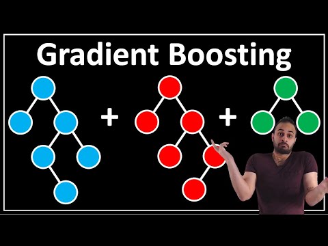
Boosting takes the opposite approach: trees are trained sequentially, each one learning from the mistakes of the ones before it.

Bagging vs. Boosting¶

	Bagging (Random Forest)	Boosting (XGBoost)
Trees trained	In parallel	Sequentially
Each tree trained on	Bootstrap sample	Residuals from previous trees
Goal	Reduce variance	Reduce bias
Risk	Overfitting (low — trees are independent)	Overfitting (if learning rate or n_estimators is too high)
Speed	Faster (parallelizable)	Slower (sequential)
Typical accuracy	Very good	Often slightly better

How does boosting learn from mistakes?¶

Train a simple tree on the original data. It makes some errors (residuals).
Train the next tree specifically to predict those residuals — the mistakes.
Add the new tree’s predictions to the previous ones. Errors shrink.
Repeat: each new tree corrects what the ensemble got wrong so far.

This is called gradient boosting because each step uses the gradient (direction of improvement) of a loss function to decide what the next tree should learn.

Note: The term “gradient” here is the same concept as in the gradient descent algorithm we saw earlier: we’re taking small steps to minimize error.

Why “learning from mistakes” needs regularization¶

Boosting works by repeatedly fitting the errors left over from previous trees. But there is a catch: if each tree is too flexible, the ensemble will start fitting noise instead of signal. Consider fitting a step function to the points below — which of the three candidates is the best fit?

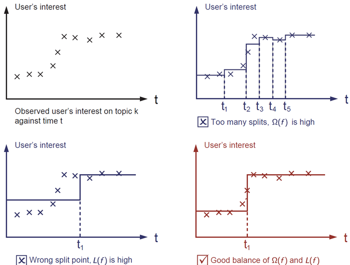
Image: XGBoost documentation — Introduction to Boosted Trees. The red model wins — it is both simple and predictive. This balance is the bias–variance tradeoff, and it is exactly what XGBoost’s regularization (which we tune in Lesson 3) controls. The top-right plot overfits by adding intermediate steps where it should model a single step function.

Visualizing Boosting: A Manual Example¶

Before using XGBoost, let’s build a simple gradient booster by hand to see exactly how residual correction works. We’ll use a very shallow tree (a “stump”) as our base learner.

# Load in the California housing dataset and split it into training and testing sets for the next section

import pandas as pd
import numpy as np
import seaborn as sns
import matplotlib.pyplot as plt
from sklearn.datasets import fetch_california_housing
from sklearn.model_selection import train_test_split
from sklearn.tree import DecisionTreeRegressor
from sklearn.ensemble import RandomForestRegressor
from sklearn.metrics import root_mean_squared_error
sns.set_theme()

housing = fetch_california_housing(as_frame=True)
df = housing.frame
X = df.drop("MedHouseVal", axis=1)
y = df["MedHouseVal"]
X_train, X_test, y_train, y_test = train_test_split(X, y, test_size=0.2, random_state=42)
print("Dataset loaded:", df.shape)

from sklearn.tree import DecisionTreeRegressor

# Step 1: Start with a very simple prediction — just the mean of y
residuals = y_train.copy()
predictions_train = np.full(len(y_train), y_train.mean())
predictions_test  = np.full(len(y_test),  y_train.mean())

# Initialize residuals as the target minus the baseline prediction
residuals = y_train - predictions_train

print(f"Baseline RMSE (predicting mean): "
      f"{root_mean_squared_error(y_test, predictions_test):.4f}\n")

learning_rate = 0.3
n_rounds = 10

for i in range(n_rounds):
    # Step 2: Train a shallow tree on the current residuals
    stump = DecisionTreeRegressor(max_depth=3, random_state=i)
    stump.fit(X_train, residuals)

    # Step 3: Update predictions and residuals
    predictions_train += learning_rate * stump.predict(X_train)
    predictions_test  += learning_rate * stump.predict(X_test)
    residuals          = y_train - predictions_train

    rmse = root_mean_squared_error(y_test, predictions_test)
    print(f"  Round {i+1:2d}: RMSE = {rmse:.4f}")

Each round, the RMSE drops as the new tree corrects the previous mistakes. This is exactly how XGBoost works — just with many more engineering optimizations that make it dramatically faster and more accurate.

Meet XGBoost¶

XGBoost (eXtreme Gradient Boosting) was developed by Tianqi Chen and released in 2014. It quickly became one of the most widely-used machine learning algorithms because:

It’s extremely fast: uses parallel processing for tree building
It regularizes automatically to prevent overfitting
It handles missing values natively
It won dozens of Kaggle competitions after its release

XGBoost is fully compatible with the sklearn API, so it works exactly like any other sklearn model.

Installation: If you get an ImportError, install with pip install xgboost or conda install -c conda-forge xgboost.

Watch: boosting, one tree at a time¶

Before we use the library, it helps to see how each tree corrects the previous ones. The video below walks through XGBoost regression from scratch — building the first prediction, computing residuals, and fitting trees to those residuals — the same loop we just coded by hand above. Note this video goes into a lot of the inner working details of XGBoost. It’s not strictly necessary to completely understand this to use it though.

Video: StatQuest with Josh Starmer — “XGBoost Part 1 (of 4): Regression” (click the thumbnail to open on YouTube). The cell below embeds it to play inline.

# Watch the boosting idea explained step by step (runs inline in Jupyter).
# StatQuest with Josh Starmer — "XGBoost Part 1 (of 4): Regression"
from IPython.display import YouTubeVideo
YouTubeVideo("OtD8wVaFm6E", width=720, height=405)

try:
    import xgboost
except ImportError:
    %pip install xgboost
    
from xgboost import XGBRegressor

xgb_reg = XGBRegressor(
    n_estimators=100,       # number of trees (boosting rounds)
    learning_rate=0.1,      # how much each tree contributes (shrinkage)
    max_depth=6,            # maximum tree depth
    random_state=42,
    verbosity=0             # suppress training output
)
xgb_reg.fit(X_train, y_train)
print(f"XGBoost RMSE: {root_mean_squared_error(y_test, xgb_reg.predict(X_test)):.4f}")

XGBoost improves on the random forest from Lesson 1. Let’s compare all models side by side.

# Train all three models
dt = DecisionTreeRegressor(max_depth=5, random_state=42).fit(X_train, y_train)
rf = RandomForestRegressor(n_estimators=100, random_state=42, n_jobs=-1).fit(X_train, y_train)
xgb = XGBRegressor(n_estimators=100, learning_rate=0.1, max_depth=6,
                   random_state=42, verbosity=0).fit(X_train, y_train)

models = {"Decision Tree": dt, "Random Forest": rf, "XGBoost": xgb}
for name, model in models.items():
    rmse = root_mean_squared_error(y_test, model.predict(X_test))
    print(f"  {name:<20} RMSE = {rmse:.4f}")

XGBoost for Classification¶

XGBoost also handles classification tasks through XGBClassifier. Let’s apply it to the breast cancer dataset from Problem 1 in the last lesson, where we predict whether a tumor is malignant (0) or benign (1).

from sklearn.datasets import load_breast_cancer
from xgboost import XGBClassifier
from sklearn.metrics import accuracy_score, classification_report

cancer = load_breast_cancer(as_frame=True)
df_c = cancer.frame
X_c = df_c.drop("target", axis=1)
y_c = df_c["target"]
X_c_tr, X_c_te, y_c_tr, y_c_te = train_test_split(X_c, y_c, test_size=0.2, random_state=42)

xgb_clf = XGBClassifier(
    n_estimators=100,
    learning_rate=0.1,
    max_depth=4,
    random_state=42,
    eval_metric="logloss",  # suppress warning about default metric
    verbosity=0
)
xgb_clf.fit(X_c_tr, y_c_tr)
preds = xgb_clf.predict(X_c_te)

print(f"XGBoost Accuracy: {accuracy_score(y_c_te, preds):.4f}\n")
print(classification_report(y_c_te, preds, target_names=cancer.target_names))

The classification_report shows us precision, recall, and F1-score for each class.

Precision: of all tumors we predicted as malignant, what fraction actually were?
Recall: of all actual malignant tumors, what fraction did we catch?
F1-score: harmonic mean of precision and recall

In a medical context, which is more important — high precision or high recall? Why?

# Compare classifiers side by side
from sklearn.ensemble import RandomForestClassifier
from sklearn.tree import DecisionTreeClassifier

models_c = {
    "Decision Tree":   DecisionTreeClassifier(random_state=42),
    "Random Forest":   RandomForestClassifier(n_estimators=100, random_state=42),
    "XGBoost":         XGBClassifier(n_estimators=100, learning_rate=0.1,
                                     random_state=42, eval_metric="logloss", verbosity=0),
}
for name, model in models_c.items():
    model.fit(X_c_tr, y_c_tr)
    acc = accuracy_score(y_c_te, model.predict(X_c_te))
    print(f"  {name:<20} Accuracy = {acc:.4f}")

Understanding XGBoost’s Key Parameters¶

You’ve seen three parameters so far. Let’s understand what they do:

`n_estimators` — number of boosting rounds¶

More rounds = more corrections = lower training error. But beyond a certain point, the model starts to overfit (memorize training noise). The right number depends on the learning_rate.

`learning_rate` — how much each tree contributes¶

Also called the shrinkage factor. A smaller learning rate means each tree takes smaller steps, requiring more trees (n_estimators) but often producing a more generalizable model.

The key trade-off: small learning_rate + large n_estimators usually wins, but takes longer to train.

# Explore the learning rate vs n_estimators trade-off
configs = [
    {"lr": 0.30, "n": 50},
    {"lr": 0.10, "n": 100},
    {"lr": 0.05, "n": 200},
    {"lr": 0.01, "n": 1000},
]

print(f"{'Learning Rate':<15} {'n_estimators':<15} {'Test RMSE':<10}")
print("-" * 40)
for cfg in configs:
    m = XGBRegressor(learning_rate=cfg["lr"], n_estimators=cfg["n"],
                     random_state=42, verbosity=0).fit(X_train, y_train)
    rmse = root_mean_squared_error(y_test, m.predict(X_test))
    print(f"  {cfg['lr']:<13} {cfg['n']:<15} {rmse:.4f}")

`max_depth` — how deep each tree grows¶

Deeper trees can capture more complex patterns but are also more likely to overfit. XGBoost trees are typically shallower than random forest trees because each tree only needs to learn a correction, not the entire signal.

# Effect of max_depth on XGBoost
depths = [2, 3, 4, 5, 6, 7, 8]
train_rmses, test_rmses = [], []

for d in depths:
    m = XGBRegressor(n_estimators=100, learning_rate=0.1, max_depth=d,
                     random_state=42, verbosity=0)
    m.fit(X_train, y_train)
    train_rmses.append(root_mean_squared_error(y_train, m.predict(X_train)))
    test_rmses.append( root_mean_squared_error(y_test,  m.predict(X_test)))

results = pd.DataFrame({
    "max_depth": depths * 2,
    "RMSE": train_rmses + test_rmses,
    "Split": ["Train"] * len(depths) + ["Test"] * len(depths)
})
sns.lineplot(results, x="max_depth", y="RMSE", hue="Split")
plt.title("XGBoost: Effect of max_depth on Train vs. Test Error")
plt.xlabel("max_depth");

Summary¶

Aspect	Random Forest	XGBoost
Strategy	Parallel bagging	Sequential boosting
Corrects	Variance	Bias and variance
Parameter emphasis	`n_estimators`, `max_features`	`learning_rate`, `n_estimators`, `max_depth`
Performance	Very good	Often better
Interpretability	Feature importances	Feature importances (+ more)

Both algorithms use decision trees as building blocks. The difference is in how those trees are combined. In the next lesson, we’ll learn how to systematically tune XGBoost’s many parameters to squeeze out the best possible performance.

Practice Problems¶

Problem 1¶

The learning_rate controls how much each tree “shrinks” its contribution. Train three XGBoost models with learning_rate values of 0.5, 0.1, and 0.01, each with 200 n_estimators. Compare their test RMSEs on the California housing data.

Which learning rate performs best? What happens when the learning rate is too high?

# TODO: Fill in the loop
for lr in [0.5, 0.1, 0.01]:
    m = XGBRegressor(n_estimators=500, learning_rate=lr, random_state=42, verbosity=0)
    m.fit(...)
    rmse = root_mean_squared_error(...)
    print(f"  learning_rate={lr}: RMSE = {rmse:.4f}")

Problem 2¶

XGBoost’s n_estimators is analogous to a random forest’s n_estimators, but they behave differently. Train both a RandomForestRegressor and an XGBRegressor for n_estimators in [10, 25, 50, 100, 200]. Plot both models’ test RMSE on the same chart.

For small n_estimators, which model performs better? What about large n_estimators? Why might this be?

n_vals = [10, 25, 50, 100, 200]
rf_rmses, xgb_rmses = [], []

for n in n_vals:
    # TODO: Train RandomForestRegressor and XGBRegressor for each n
    rf_m  = ...
    xgb_m = ...
    rf_rmses.append(root_mean_squared_error(y_test, rf_m.predict(X_test)))
    xgb_rmses.append(root_mean_squared_error(y_test, xgb_m.predict(X_test)))

results = pd.DataFrame({
    "n_estimators": n_vals * 2, # Create a column with n_estimators repeated for both models
    "RMSE": rf_rmses + xgb_rmses,
    "Model": ["Random Forest"] * len(n_vals) + ["XGBoost"] * len(n_vals)
})
# TODO: Plot results using sns.lineplot

Problem 3¶

Apply XGBClassifier to the breast cancer dataset and produce a confusion matrix to understand which tumors the model misclassifies. A confusion matrix shows true positives, true negatives, false positives, and false negatives.

Why is a false negative (predicting benign when it’s actually malignant) more costly than a false positive in a cancer screening context?

from sklearn.metrics import ConfusionMatrixDisplay

# The classifier clf from above (re-train if needed)
xgb_clf = XGBClassifier(n_estimators=100, learning_rate=0.1, max_depth=4,
                        random_state=42, eval_metric="logloss", verbosity=0)
xgb_clf.fit(X_c_tr, y_c_tr)

# TODO: Create and display a confusion matrix